Analyzing Patient Data

Overview

Teaching: 30 min
Exercises: 0 min

Questions

• How can I process and visualize my data?

Objectives

• Navigate among important sections of the MATLAB environment.

• Identify what kind of data is stored in MATLAB arrays.

• Read tabular data from a file into a program.

• Assign values to variables.

• Select individual values and subsections from data.

• Perform operations on arrays of data.

• Display simple graphs.

We are studying inflammation in patients who have been given a new treatment for arthritis, and need to analyze the first dozen data sets. The data sets are stored in Comma Separated Values (CSV) format: each row holds information for a single patient, and the columns represent successive days. The first few rows of our first file, inflammation-01.csv, look like this:

0,0,1,3,1,2,4,7,8,3,3,3,10,5,7,4,7,7,12,18,6,13,11,11,7,7,4,6,8,8,4,4,5,7,3,4,2,3,0,0
0,1,2,1,2,1,3,2,2,6,10,11,5,9,4,4,7,16,8,6,18,4,12,5,12,7,11,5,11,3,3,5,4,4,5,5,1,1,0,1
0,1,1,3,3,2,6,2,5,9,5,7,4,5,4,15,5,11,9,10,19,14,12,17,7,12,11,7,4,2,10,5,4,2,2,3,2,2,1,1
0,0,2,0,4,2,2,1,6,7,10,7,9,13,8,8,15,10,10,7,17,4,4,7,6,15,6,4,9,11,3,5,6,3,3,4,2,3,2,1
0,1,1,3,3,1,3,5,2,4,4,7,6,5,3,10,8,10,6,17,9,14,9,7,13,9,12,6,7,7,9,6,3,2,2,4,2,0,1,1

We want to:

• load that data into memory,
• calculate the average inflammation per day across all patients, and
• plot the result.

To do all that, we’ll have to learn a little bit about programming.

Introduction to the MATLAB GUI

Before we can start programming, we need to know a little about the MATLAB interface. Using the default setup, the MATLAB desktop contains several important sections:

• In the Command Window we can run and debug our code. Everything that’s typed into the command window is executed immediately.
• Alternatively, we can open the Editor, write our code and run it all at once. The upside of this is that we can save our code and run it again in the same way at a later stage.
• The Workspace contains all the variables which we have loaded into memory.
• The Current Folder window shows files in the current directory, and we can change the current folder using this window.
• Search Documentation on the top right of your screen lets you search for functions. Suggestions for functions that would do what you want to do will pop up. Clicking on them will open the documentation. Another way to access the documentation is via the help command — we will return to this later.

Good practices for project organisation

Before we get started, let’s create some directories to help organise this project.

Tip: Good Enough Practices for Scientific Computing

Good Enough Practices for Scientific Computing gives the following recommendations for project organization:

1. Put each project in its own directory, which is named after the project.
2. Put text documents associated with the project in the doc directory.
3. Put raw data and metadata in the data directory, and files generated during clean-up and analysis in a results directory.
4. Put source code for the project in the src directory, and programs brought in from elsewhere or compiled locally in the bin directory.
5. Name all files to reflect their content or function.

We already have a data directory in our matlab-novice-inflammation project directory, so we only need to create a results directory for this project. You can use your computer’s file browser to create this directory. We’ll save all our scripts and function files in the main project directory.

A final step is to set the current folder in MATLAB to our project folder. Use the Current Folder window in the MATLAB GUI to browse to your project folder (matlab-novice-inflammation).

In order to check the current directory, we can run pwd to print the working directory. A second check we can do is to run the ls command in the Command Window — we should get the following output:

data   results

Reading data from files and writing data to them are essential tasks in scientific computing, and admittedly, something that we’d rather not spend a lot of time thinking about. Fortunately, MATLAB comes with a number of high-level tools to do these things efficiently, sparing us the grisly detail.

If we know what our data looks like (in this case, we have comma-separated values) and we’re unsure about what command we want to use, we can search the documentation.
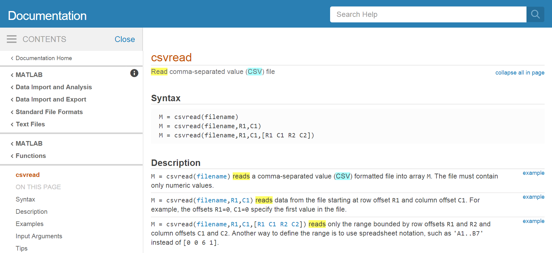
Type read csv into the documentation toolbar. We can refine by Category (facets on the left) to focus on MATLAB documentation only. MATLAB suggests using read and csvread. We will choose csvread in this case because it is more specific to our needs to read csv files. If we have a closer look at the documentation, MATLAB tells us which in- and output arguments this function has.

To load the data from our CSV file into MATLAB, type the following command into the MATLAB command window, and press Enter:

csvread('data/inflammation-01.csv')

You should see a wall of numbers on the screen—these are the values from the CSV file. It can sometimes be useful to see the output from MATLAB commands, but it is often not. To suppress the output, put a semicolon at the end of your command:

csvread('data/inflammation-01.csv');

The expression csvread(...) is a function call. Functions generally need arguments to run. In the case of the csvread function, we need to provide a single argument: the name of the file we want to read data from. This argument needs to be a character string or string, so we put it in quotes.

Our call to csvread read our file, and printed the data inside to the screen. Adding a semicolon avoided the numbers to show in the screen. The data, in both cases, was saved to an automatically generated variable named ans. You can see it in the Workspace. The variable ans will save the most recent answer when you don’t specify an output argument. This means that next time you type an operation without an output argument the value of ans will change. This will make operating with the data difficult and confusing, we need to assign the array to a variable.

patient_data = csvread('data/inflammation-01.csv');

A variable is just a name for a piece of data or value. Variable names must begin with a letter, and can contain numbers or underscores. Examples of valid variable names are x, f_0 or current_temperature.

We can create a new variable simply by assigning a value to it using =:

weight_kg = 55;

Once a variable has a value, we can print it using the disp function:

disp(weight_kg)

55

or simply typing its name, followed by Enter

weight_kg

w =
    55

and do arithmetic with it:

weight_lb = 2.2 * weight_kg;
disp(['Weight in pounds: ', num2str(weight_lb)])

Weight in pounds: 121

The disp function takes a single argument – the value to print. To print more than one value on a single line, we could print an array of values. All values in this array need to be the same type. So, if we want to print a string and a numerical value together, we have to convert that numerical value to a string with the num2str function.

Assignment is giving a name to a value so that it can be used again, and accessed by other parts of a program.

Assigning a value to one variable does not change the values of other variables. For example,

weight_kg = 57.5;
weight_lb = 2.2 * weight_kg;
disp(['Weight in kg: ', num2str(weight_kg)])
disp(['Weight in pounds: ', num2str(weight_lb)])

Weight in kg: 57.5
Weight in pounds: 126.5

Let’s update the value of one of our variables, and print the values of both:

weight_kg = 100;
disp(['Weight in kg: ', num2str(weight_kg)])
disp(['Weight in pounds: ', num2str(weight_lb)])

Weight in kg: 100
Weight in pounds: 126.5

Since weight_lb doesn’t “remember” where its value came from, it isn’t automatically updated when weight_kg changes. This is important to remember, and different from the way spreadsheets work.

Now that we know how to assign values to variables, let’s view a list of all the variables in our workspace:

who

Your variables are:

ans patient_data  weight_kg  weight_lb

To remove a variable from MATLAB, use the clear command:

clear weight_lb
who

Your variables are:

patient_data  weight_kg

Alternatively, we can look at the Workspace. The workspace contains all variable names and assigned values that we currently work with. As long as they pop up in the workspace, they are universally available. It’s generally a good idea to keep the workspace as clean as possible. To remove all variables from the workspace, execute the command clear all.

Predicting Variable Values

Predict what variables refer to what values after each statement in the following program:

mass = 47.5
age = 122
mass = mass * 2.0
age = age - 20

Now that our data is in memory, we can start doing things with it. First, let’s find out its size:

size(patient_data)

ans =

    60 40

The output tells us that the variable patient_data refers to a table of values that has 60 rows and 40 columns.

MATLAB stores all data in the form of multi-dimensional arrays. For example:

• Numbers, or scalars are represented as two dimensional arrays with only one row and one column, as are single characters.
• Lists of numbers, or vectors are two dimensional as well, but the value of one of the dimensions equals one. By default vectors are row vectors, meaning they have one row and as many columns as there are elements in the vector.
• Tables of numbers, or matrices are arrays with more than one column and more than one row.
• Even character strings, like sentences, are stored as an “array of characters”.

Normally, MATLAB arrays can’t store elements of different data types. For instance, a MATLAB array can’t store both a float and a char. To do that, you have to use a Cell Array.

We can use the class function to find out what kind of data lives inside an array:

class(patient_data)

ans = double

This output tells us that patient_data refers to an array of double precision floating-point numbers. This is the default numeric data type in MATLAB. If you want to store other numeric data types, you need to tell MATLAB explicitly. For example, the command,

x = int16(325);

assigns the value 325 to the name x, storing it as a 16-bit signed integer.

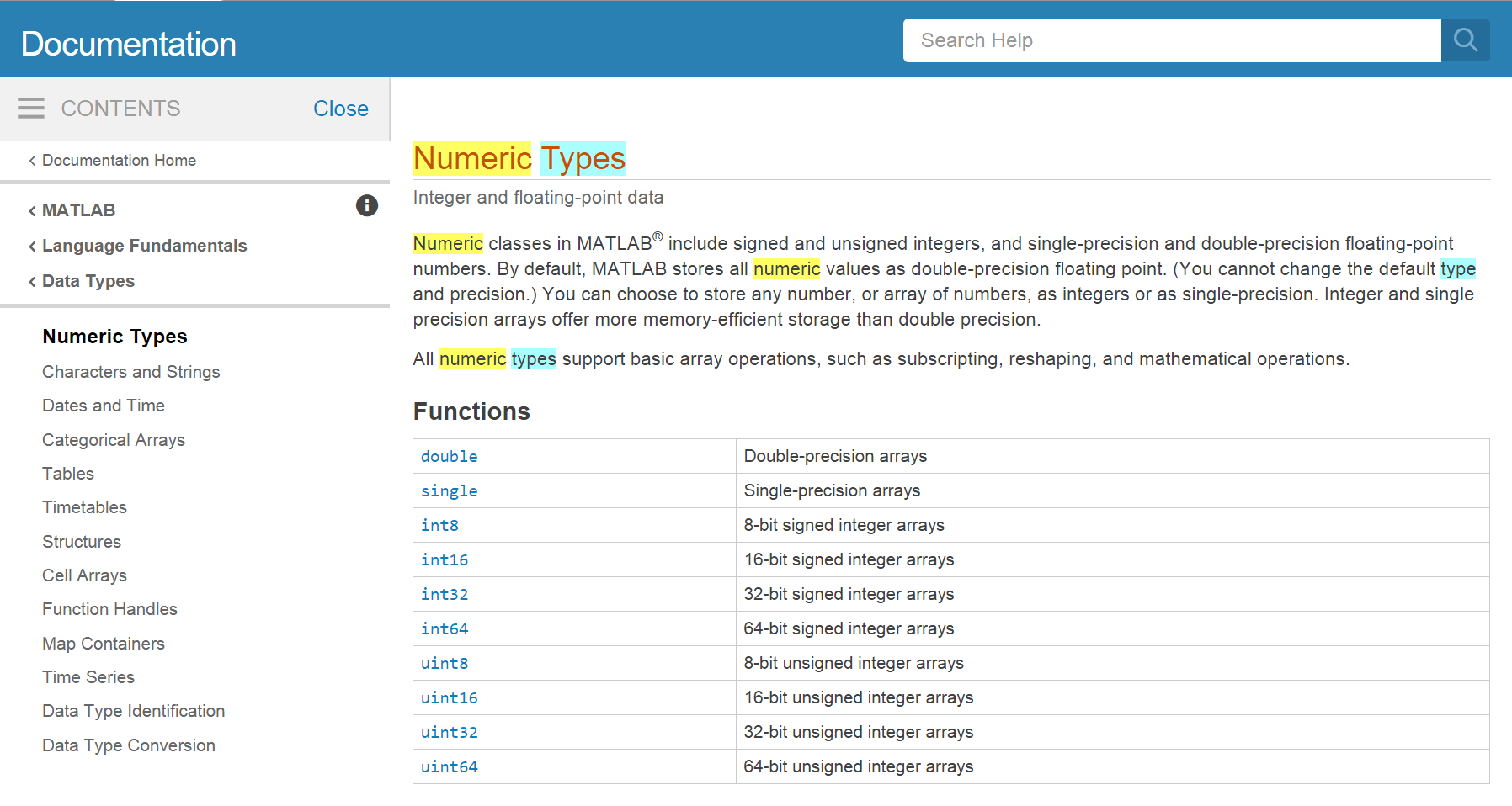
To learn more about numeric data types you can type Numeric Types in the search box. We will use the Matlab default (double precision floating-point) during this workshop. The number type will affect the precision of your calculations and the memory and execution time of Matlab.

Let’s work on selecting values from a matrix in Matlab. We will create an 8-by-8 “magic” Matrix. A magic matrix has some special properties, but here we will just use it as an example of a matrix with random numbers (if you want to learn more about magic matrix, search magic in the search box!):

M = magic(8)

ans =

   64    2    3   61   60    6    7   57
    9   55   54   12   13   51   50   16
   17   47   46   20   21   43   42   24
   40   26   27   37   36   30   31   33
   32   34   35   29   28   38   39   25
   41   23   22   44   45   19   18   48
   49   15   14   52   53   11   10   56
    8   58   59    5    4   62   63    1

We want to access a single value from the matrix:

To do that, we must provide its index in parentheses:

M(5, 6)

ans = 38

Indices are provided as (row, column). So the index (5, 6) selects the element on the fifth row and sixth column.

An index like (5, 6) selects a single element of an array, but we can also access sections of the matrix, or slices. To access a row of values:

we can do:

M(5, :)

ans =

   32   34   35   29   28   38   39   25

Providing : as the index for a dimension selects all elements along that dimension. So, the index (5, :) selects the elements on row 5, and all columns—effectively, the entire row. We can also select multiple rows,

M(1:4, :)

ans =

   64    2    3   61   60    6    7   57
    9   55   54   12   13   51   50   16
   17   47   46   20   21   43   42   24
   40   26   27   37   36   30   31   33

and columns:

M(:, 6:end)

ans =

    6    7   57
   51   50   16
   43   42   24
   30   31   33
   38   39   25
   19   18   48
   11   10   56
   62   63    1

To select a submatrix,

we have to take slices in both dimensions:

M(4:6, 5:7)

ans =

   36   30   31
   28   38   39
   45   19   18

We don’t have to take all the values in the slice—if we provide a stride. Let’s say we want to start with row 2, and subsequently select every third row:

M(2:3:end, :)

ans =

    9   55   54   12   13   51   50   16
   32   34   35   29   28   38   39   25
    8   58   59    5    4   62   63    1

Slicing

A subsection of an array is called a slice. We can take slices of character strings as well:

element = 'oxygen';
disp(['first three characters: ', element(1:3)])
disp(['last three characters: ', element(4:6)])

first three characters: oxy
last three characters: gen

1. What is the value of element(4:end)? What about element(1:2:end)? Or element(2:end - 1)?

2. For any size array, MATLAB allows us to index with a single colon operator (:). This can have surprising effects. For instance, compare element with element(:). What is size(element) versus size(element(:))? Finally, try using the single colon on the matrix M above: M(:). What seems to be happening when we use the single colon operator for slicing?

Now that we know how to access data we want to compute with, we’re ready to analyze patient_data. MATLAB knows how to perform common mathematical operations on arrays. If we want to find the average inflammation for all patients on all days, we can just ask for the mean of the array:

mean(patient_data(:))

ans = 6.1487

If we did mean(patient_data) , that would compute the mean of each column in our table, and return an array of mean values. The expression patient_data(:) flattens the table into a one-dimensional array.

To get details about what a function, like mean, does and how to use it, we can search the documentation, or use MATLAB’s help command.

help mean

mean   Average or mean value.
    S = mean(X) is the mean value of the elements in X if X is a vector. 
    For matrices, S is a row vector containing the mean value of each 
    column. 
    For N-D arrays, S is the mean value of the elements along the first 
    array dimension whose size does not equal 1.
 
    mean(X,DIM) takes the mean along the dimension DIM of X.
 
    S = mean(...,TYPE) specifies the type in which the mean is performed, 
    and the type of S. Available options are:
 
    'double'    -  S has class double for any input X
    'native'    -  S has the same class as X
    'default'   -  If X is floating point, that is double or single,
                   S has the same class as X. If X is not floating point, 
                   S has class double.
 
    S = mean(...,NANFLAG) specifies how NaN (Not-A-Number) values are 
    treated. The default is 'includenan':
 
    'includenan' - the mean of a vector containing NaN values is also NaN.
    'omitnan'    - the mean of a vector containing NaN values is the mean 
                   of all its non-NaN elements. If all elements are NaN,
                   the result is NaN.
 
    Example:
        X = [1 2 3; 3 3 6; 4 6 8; 4 7 7]
        mean(X,1)
        mean(X,2)
 
    Class support for input X:
       float: double, single
       integer: uint8, int8, uint16, int16, uint32,
                int32, uint64, int64
 
    See also median, std, min, max, var, cov, mode.

We can also compute other statistics, like the maximum, minimum and standard deviation.

disp(['Maximum inflammation: ', num2str(max(patient_data(:)))])
disp(['Minimum inflammation: ', num2str(min(patient_data(:)))])
disp(['Standard deviation: ', num2str(std(patient_data(:)))])

Maximum inflammation: 20
Minimum inflammation: 0
Standard deviation: 4.6148

When analyzing data, though, we often want to look at partial statistics, such as the maximum value per patient or the average value per day. One way to do this is to assign the data we want to a new temporary array, then ask it to do the calculation:

patient_1 = patient_data(1, :)
disp(['Maximum inflation for patient 1: ', num2str(max(patient_1))])

Maximum inflation for patient 1: 18

We don’t actually need to store the row in a variable of its own. Instead, we can combine the selection and the function call:

max(patient_data(1, :))

ans = 18

What if we need the maximum inflammation for all patients, or the average for each day? As the diagram below shows, we want to perform the operation across an axis:

To support this, MATLAB allows us to specify the dimension we want to work on. If we ask for the average across the dimension 1, we get:

mean(patient_data, 1)

ans =

 Columns 1 through 13:

    0.00000    0.45000    1.11667    1.75000    2.43333    3.15000    3.80000    3.88333    5.23333    5.51667    5.95000    5.90000    8.35000

 Columns 14 through 26:

    7.73333    8.36667    9.50000    9.58333   10.63333   11.56667   12.35000   13.25000   11.96667   11.03333   10.16667   10.00000    8.66667

 Columns 27 through 39:

    9.15000    7.25000    7.33333    6.58333    6.06667    5.95000    5.11667    3.60000    3.30000    3.56667    2.48333    1.50000    1.13333

 Column 40:

    0.56667

As a quick check, we can check the size of this array:

size(mean(patient_data, 1))

ans =
    1    40

The size tells us we have a 1-by-40 vector, so this is the average inflammation per day for all patients. Let’s save this vector as a variable:

ave_day=mean(patient_data,1);

If we average across axis 2, we get the average inflammation per patient across all days.:

ave_patient = mean(patient_data, 2)

ave_patient =

   5.4500
   5.4250
   6.1000
   5.9000
   5.5500
   6.2250
   5.9750
   6.6500
   6.6250
   6.5250
   6.7750
   5.8000
   6.2250
   5.7500
   5.2250
   6.3000
   6.5500
   5.7000
   5.8500
   6.5500
   5.7750
   5.8250
   6.1750
   6.1000
   5.8000
   6.4250
   6.0500
   6.0250
   6.1750
   6.5500
   6.1750
   6.3500
   6.7250
   6.1250
   7.0750
   5.7250
   5.9250
   6.1500
   6.0750
   5.7500
   5.9750
   5.7250
   6.3000
   5.9000
   6.7500
   5.9250
   7.2250
   6.1500
   5.9500
   6.2750
   5.7000
   6.1000
   6.8250
   5.9750
   6.7250
   5.7000
   6.2500
   6.4000
   7.0500
   5.9000

The mathematician Richard Hamming once said, “The purpose of computing is insight, not numbers,” and the best way to develop insight is often to visualize data. Visualization deserves an entire lecture (or course) of its own, but we can explore a few features of MATLAB here.

Let’s take a look at the average inflammation over time:

figure
ave_day = mean(patient_data, 1);
plot(ave_day)
title('Daily average inflammation')
xlabel('Day of trial')
ylabel('Inflammation')

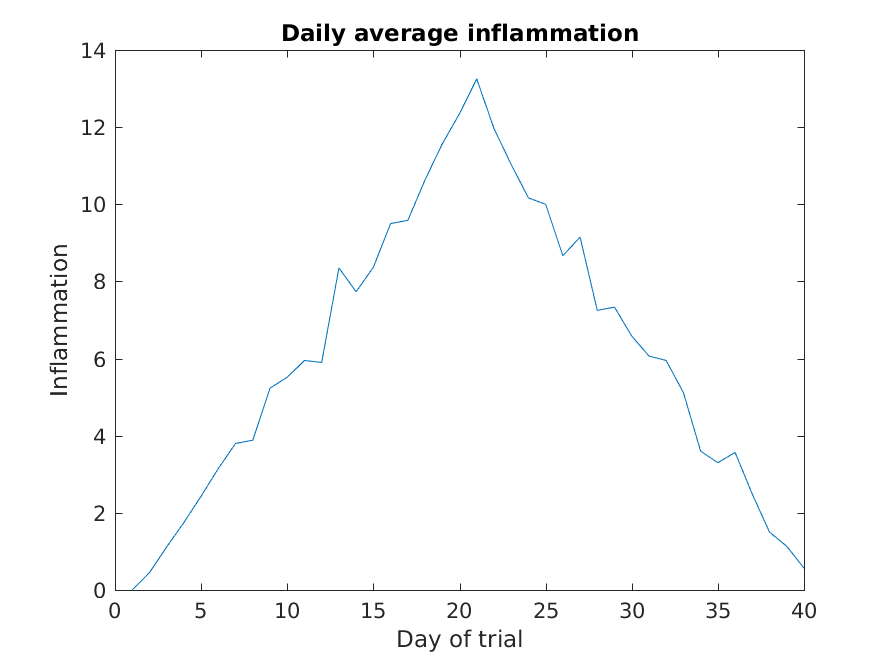
Here, we have put the average per day across all patients in the variable ave_day, then used the plot function to display a line graph of those values.

It’s good practice to give the figure a title, and to label the axes using xlabel and ylabel so that other people can understand what it shows (including us if we return to this plot 6 months from now).

The result is roughly a linear rise and fall, which is suspicious: based on other studies, we expect a sharper rise and slower fall. Let’s have a look at two other statistics: the maximum and minimum inflammation per day across all patients.

Let’s take a look first at how the max function works with matrices.

help max

max    Largest component.
    For vectors, max(X) is the largest element in X. For matrices,
    max(X) is a row vector containing the maximum element from each
    column. For N-D arrays, max(X) operates along the first
    non-singleton dimension.
    
    (...)

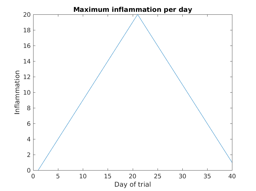
So, using max directly will work in our case, because we want the maximums of each column to get the maximum inflammation per day.

figure
plot(max(patient_data))
title('Maximum inflammation per day')
title('Daily average inflammation')
ylabel('Inflammation')
xlabel('Day of trial')

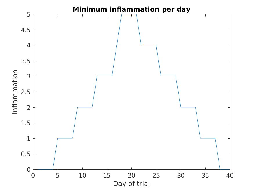
figure
plot(min(patient_data, [], 1))
title('Minimum inflammation per day')
ylabel('Inflammation')
xlabel('Day of trial')

Like mean(), the functions max() and min() can also operate across a specified dimension of the matrix. However, the syntax is slightly different. To run max() or min() for other dimensions the

To see why, run a help on each of these functions.

From the figures, we see that the maximum value rises and falls perfectly smoothly, while the minimum seems to be a step function. Neither result seems particularly likely, so either there’s a mistake in our calculations or something is wrong with our data.

Plots

When we plot just one variable using the plot command e.g. plot(Y) what do the x-values represent?

Solution

The x-values are the indices of the y-data, so the first y-value is plotted against index 1, the second y-value against 2 etc.

Why are the vertical lines in our plot of the minimum inflammation per day not perfectly vertical?

Solution

MATLAB interpolates between the points on a 2D line plot.

Create a plot showing the standard deviation of the inflammation data for each day across all patients. Hint: search the documentation for standard deviation

Solution

plot(std(patient_data, 0, 2))
xlabel('Day of trial')
ylabel('Inflammation')
title('Standard deviation across all patients')

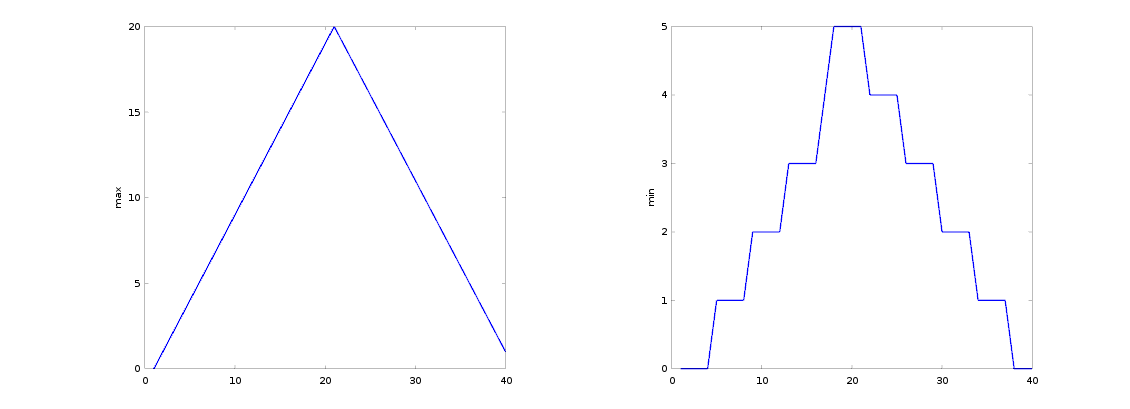
It is often convenient to combine multiple plots into one figure using the subplotcommand which plots our graphs in a grid pattern. The first two parameters describe the grid we want to use, while the third parameter indicates the placement on the grid.

figure

subplot(1, 2, 1)
plot(max(patient_data, [], 1))
ylabel('max')

subplot(1, 2, 2)
plot(min(patient_data, [], 1))
ylabel('min')

We can also plot 2 dimensional data with Matlab. Let’s display a heat map of our data:

figure
imagesc(patient_data)
title('Inflammation')
xlabel('Day of trial')
ylabel('Patient number')

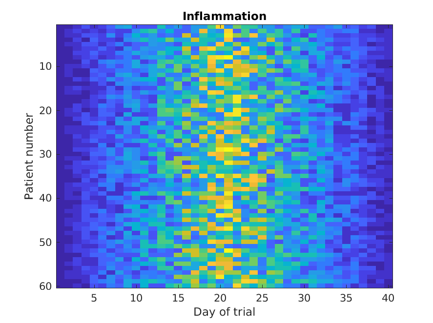
The imagesc function represents the matrix as a color image. Every value in the matrix is mapped to a color. Blue regions in this heat map are low values, while yellow shows high values. As we can see, inflammation rises and falls over a 40 day period.

Our work so far has convinced us that something is wrong with our first data file. We would like to check the other 11 the same way, but typing in the same commands repeatedly is tedious and error-prone. Since computers don’t get bored (that we know of), we should create a way to do a complete analysis with a single command, and then figure out how to repeat that step once for each file. These operations are the subjects of the next two lessons.

Key Points

• MATLAB stores data in arrays.

• Use csvread to read tabular CSV data into a program.

• Use plot to visualize data.